R Days in Rennes, France

The R Days, the annual event around R in France, was held this year in Rennes.

You can get the abstract for the talk I made around the use of AI to predict network saturation.

& or &&, that is the question

The R language has two AND operators: & and &&. Knowing the difference is key when working with if clauses.

The R documentation states that:

The longer form the left to right examining only the first element of each vector. Evaluation proceeds only until the result is determined. The longer form is appropriate for programming control-flow and typically preferred in if clauses.<

Consider the following variables:

x = c(1, 2)
y = c(2, 1)

The code below produces a logical vector of size 2: the evaluation is done for each of the elements.

x == 1 & y == 1

## [1] FALSE FALSE

The second example below ends up testing the first element of each vector (i.e. x[[1]] == 1 & y[[1]] == 1) and produces a single value (TRUE & FALSE = FALSE).

x == 1 && y == 1

## [1] FALSE

The last example produces TRUE as both the first value of x is equal to 1 and the first value of y is equal to 2.

x == 1 && y == 2

## [1] TRUE

Note that if the comparison is done on vectors of different lengths, operator & will throw a warning.

z = c(1, 2, 3)
x == 1 & z == 2

## Warning in x == 1 & z == 2: longer object length is not a multiple of
## shorter object length

## [1] FALSE FALSE FALSE

Operator && will not complain.

x == 1 && z == 2

## [1] FALSE

Back-up Anki with Dropbox

Anki is one of the best applications to help structure your learning with flash cards. Anki Web comes as a complement as it backs up your decks and cards on the cloud and enables to study on multiple synchronized devices (computers and phones). Anki Web has a retention period of 3 months: if you do not use the service for more than 3 months, your decks are deleted from the cloud. You end up then relying on the local version(s) on your device(s).

In this post, I wanted to share my experience to ensure a consistent and reliable back-up of the Anki decks using dropbox on Windows.

Rolling median with Azure Data Lake Analytics

Azure Data Lake Analytics (DLA in short) provides a rich set of analytics functions to compute an aggregate value based on a group of rows. The typical example is with the rolling average over a specific window. Below is an example where the window is centered and of size 11 (5 preceding, the current row, and 5 following). The grouping is made over the site field.

   SELECT 
        AVG(value) OVER(PARTITION BY site ORDER BY timestamp ROWS BETWEEN 5 PRECEDING AND 5 FOLLOWING) AS rolling_avg
    FROM @Data;

However, the median function does not support the ROWS option. It is not possible therefore to run rolling median straight out of the box with DLA.

 PERCENTILE_DISC(0.5) WITHIN GROUP(ORDER BY value) OVER(PARTITION BY site, timestamp ROWS BETWEEN 5 PRECEDING AND 5 FOLLOWING) AS rolling_median // will generate an error

The aim of this post is to:

• show you how the running median can be calculated on ADL by using a mix of basic JOIN
• discuss the finer points of the median functions in ADL
• compare a R implementation

Custom sorting with DT

I came across a practical case a couple of days ago where the row and column ordering provided out of the box by the R DT package was not enough.

The DT package provides a wrapper around the DataTable javascript library powered by jQuery. DT can be used in Rmarkdown documents as well as in Shiny.

The goal was to display a table containing columns reporting the bandwidth consumption for some sites. The bandwidth is expressed in bits per second (bps). When quantifying large bit rates, decimal prefixes are used. For example:

• 1,000 bps = 1 Kbps (one kilobit or one thousand bits per second)
• 1,000,000 bps = 1 Mbps (one megabit or one million bits per second)
• 1,000,000,000 bps = 1 Gbps (one gigabit or one billion bits per second)

The first approch was to take the numeric value and convert it as a string using R. This is a basic implementation:

# stringr and dplyr are loaded

set.seed(24323)
v = as.integer(runif(5, min = 10, max = 2000000))
v = c(0, 1, v) # add special cases such as 0bps, 1bps
log_base = 1000 # could be 1024 if the values need to be expressed in KB, MB, etc.

raw_base = if_else(v == 0, as.numeric(NA), trunc(log(v)/log(log_base)))
base = if_else(raw_base > 5, 5, raw_base) # we go up to PETA
   
adjusted_value = if_else(is.na(base), v, v / log_base ^ base)
unit_prefix = dplyr::case_when(
  base == 0 | is.na(base) ~ "",
  base == 1 ~ "k",
  base == 2 ~ "M",
  base == 3 ~ "G",
  base == 4 ~ "T",
  base == 5 ~ "P",
  T ~ "ERROR"
)

unit = str_c(unit_prefix, "bps")
adjusted_value_rounded = round(adjusted_value, 2) # two-digits maximum (enable to round to value above)

output = case_when(
  adjusted_value == 0 ~ str_c('0.00 ', unit),
  adjusted_value_rounded == 0 ~ str_c('< 0.01 ', unit),
  T ~ str_trim(str_c(format(adjusted_value_rounded, big.mark=',', digits=2), ' ', unit))
)

The underlying values (variable v) are as follows:

## [1]       0       1 1541474 1479601  875475  989313   92589

The converted values (variable output) are as follows:

## [1] "0.00 bps"   "1.0 bps"    "1.5 Mbps"   "1.5 Mbps"   "875.5 kbps"
## [6] "989.3 kbps" "92.6 kbps"

The data are then combined in a data frame:

dataframe = tbl_df(data.frame(
  consumption_raw = v,
  consumption_formatted = output,
  stringsAsFactors = F
)) 

When the data frame is rendered with DT with the formatted bandwidth pre-sorted, the ordering is done on the character values. So 980kbps will appear above 1.5Mpbs despite representing a smaller amount.

dataframe %>%
  DT::datatable(options = list(order = list(list(2, 'desc'))))

One way to fix it would be to sort the dataframe in R and disable sorting with DT. This approach could be frustrating for the users if the table is being viewed through Shiny.

 dataframe %>%
  arrange(desc(consumption_raw)) %>%
  DT::datatable(options = list(ordering=F))

We could use column rendering, where the raw values will be passed to the datatable and the conversion will be done in javascript. In this approach, we are basically replicating the formatting code done in R for javascript (code inspired by the following gist.

dataframe %>%
datatable(options = list(
  order = list(list(1, 'desc')),
  columnDefs = list(list(
  targets = 1,
  render = JS(
    "function(data, type, row, meta) {
         if (type != 'display') {
            return data;
         }
         var sizes = ['bps', 'kbps', 'Mbps', 'Gbps', 'Tbps'];
         if (data == 0) return '0';
         var base = parseInt(Math.floor(Math.log(data) / Math.log(1000)));
         return (data / Math.pow(1000, base)).toFixed(1) + ' ' + sizes[base];
    }")
))))

This apprach has some drawbacks:

• javacript needs to be used. Implementing JavaScript functions for people coding in R may take some times.
• Code may be duplicated as the R implementation still needs to be required (for example, if I want to include )

Another approach would be do pass to DT two values within a cell:

• the underlying raw value (an integer)
• the formatted value regarding the bandwidth consumption

• the pair can be separated by a special character such as *

  *,

The underlying raw value is used for sorting, while the formatted value will be used for display.

dataframe %>%
  mutate(
     dual_column = str_c(consumption_raw, "|", consumption_formatted) 
   ) %>% 
  datatable(options = list(
    order = list(list(3, 'desc')),
    columnDefs = list(list(
    targets = 3,
    render = JS(
      "function(data, type, row, meta) {
          split = data.split('|')
          if (type == 'display' || type == 'filter') {
            return split[1];
          } else {
            return split[0];
          }
      }")
  ))))

The trick here is to use the different values of the type parameter of the column rendering. Based on the documentation, the value can be:

• filter. This is being used by the search box. In the implementation below, the value being searched is the same as being displayed.
• display. Here, we used the second component of the string as the displayed value.
• type
• sort. Here, we used the first componen

This approach is purely client-side. When the datatable is included in Rmarkdown document or is generated by Shiny with the server-side disabled, it will work.

But when the datatable is generated using Shiny such as:

 output$table = DT::renderDataTable({
    DT::datatable(dataframe)
  }, server = T)

it will not work. When looking at the implementation, the filtering and the sorting is done in R. As you can see, when sorting an integer converted in string, R will consider that the value "10" is lower than the value "2".

v = as.character(c(1, 2, 10, 20))
sort(v)

## [1] "1"  "10" "2"  "20"

One way to fix it is adjust the first value of the pair by padding it with zero. It works well only for integer value. If you deal with numeric values, you need to make sure that all the numbers have the same number of characters to the left and to the right of the digit.

v.adj = str_pad(v, width = max(str_length(v)), side = "left", pad = "0")
sort(v.adj)

## [1] "01" "02" "10" "20"

The following adjusted code should now work in a shiny-based environment:

padding_left = max(str_length(dataframe$consumption_raw))


dataframe %>%
   mutate(
     consumption_raw = str_pad(consumption_raw, width = padding_left, side = "left", pad = "0"),
     dual_column = str_c(consumption_raw, "|", consumption_formatted),
     dual_column_render = dual_column
   ) %>% 
select(
  consumption_raw, consumption_formatted, dual_column, dual_column_render
) %>%
datatable(options = list(
  order = list(list(4, 'desc')),
  columnDefs = list(list(
  targets = 4,
  render = JS(
    "function(data, type, row, meta) {
        split = data.split('|')
        if (type == 'display') {
          return split[1];
        } else {
          return split[0];
        }
    }")
))))

R Days in Anglet

The R Days took place at the end of June 2017 in Anglet, France. The slides of the various presentations have been made public on github

Big Data Paris 2017

The conference BigData Paris was recently organized the 6th and 7th of March 2017. I though I would share my notes regarding some of the talks I attended.

Load files in R with specific encoding

When working with flat files, encoding needs to be factored in right away to avoid issues down the line. UTF-8 (or UTF-16) is the de facto encoding that you hope to get. If the encoding is different, pay attention on how you load the file into R.

Let’s take the example of a file encoded as Windows-1252. Its content is displayed below using Notepad++. The editor does a pretty good job figuring out the encoding of the file. The encoding is displayed in the status bar while the Encoding menu enables you to change the selected character set.

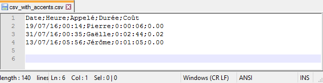
Foundations of Service Level Management: Book Review

I wanted to share a couple of notes I have made while reading Foundations of Service Level Management by Sturm, Morris, and Jander.

The book, written in the ’00s, deals with all the aspects of Service Level Management. More specifically, it covers topics such as measurement, how the SLA are defined, human challenges, best practices, etc.

The book is not technical at all and is overall an easy read. The first part of the book is generic to be relevant in years to come. Chapter 9 is worth a read as it covers what the customer could do before contacting a service center that delivers managed services.

Distinguish between a base and a SPD library

In SAS, a library engine is an engine that accesses groups of files and puts them into a logical form for processing. The engine used by default is the base engine. In addition, you may come across other engines, such as the SPD engine.

The SAS Scalable Performance Data Engine (SPD Engine) provides parallel I/O as each SAS dataset is split over multiple disks. The structure of this engine allows a faster processing of large data.

A common production set-up may define different libraries with different purposes, and therefore different engines. A library with the base engine may be used for ad-hoc reporting and small data transformation, while the library with the SPD engine may be used to store a large data mart. From a user’s perspective, the layer provided by the SAS meta-data server hides the underlying engines used by the various libraries. It is however useful to validate the type of engine being used without relying on the IT department.